Implicit Wiener Series for Higher-Order Image Analysis.
 The computation of classical higher-order statistics such as higher-order moments or spectra is difficult for images due to the huge number of terms to be estimated and interpreted. We propose an alternative approach in which multiplicative pixel interactions are described by a series of Wiener functionals. Since the functionals are estimated implicitly via polynomial kernels, the combinatorial explosion associated with the classical higher-order statistics is avoided.
Volterra and Wiener series
In system identification, one tries to infer the functional relationship between system input and output from observations of the in- and outgoing signals. If the system is linear, it can be characterized uniquely by measuring its impulse response, for instance by reverse correlation. For nonlinear systems, however, there exists a whole variety of system representations. One of them, the Wiener expansion, has found a somewhat wider use in neuroscience since its estimation constitutes a natural extension of linear system identification. The coefficients of the Wiener expansion can be estimated by a cross-correlation procedure that is conveniently applicable to experimental data.
Unfortunately, the estimation of the Wiener expansion by cross-correlation suffers from severe problems:
- In practice, the cross-correlations have to be estimated at a finite resolution. The number of expansion coefficients increases with mn for an m-dimensional input signal and an nth-order Wiener kernel such that the resulting numbers are huge for higher-order Wiener kernels. For instance, a 5th-order Wiener kernel operating on 16 x 16 sized image patches contains roughly 1012 coefficients, 1010 of which would have to be measured individually by cross-correlation. As a consequence, this procedure is not feasible for higher-dimensional input signals.
- The estimation of cross-correlations requires large sample sizes. Typically, one needs several tens of thousands of input-output pairs before a sufficient convergence is reached.
- The estimation via cross-correlation works only if the input is Gaussian noise with zero mean, not for general types of input.
- The crosscorrelation method assumes noise-free signals. For real, noise-contaminated data, the estimated Wiener series models both signal and noise of the training data which typically results in reduced prediction performance on independent test sets.
A brief tutorial on Volterra and Wiener series can be found in
[1] Franz, M.O. and B. Schölkopf: Implicit Wiener Series. MPI Technical Report (114), Max Planck Institute for Biological Cybernetics, Tübingen, Germany (June 2003) [PDF].
Implicit estimation via polynomial kernels
We propose a new estimation method based on regression in a reproducing kernel Hilbert space (RKHS) to overcome these problems. Instead of estimating each expansion coefficient individually by cross-correlation, we treat the Wiener series as a linear operator in the RKHS formed by the monomials of the input. The Wiener expansion can be found by computing the linear operator in the RKHS that minimizes the mean square error. Since the basis functions of the Wiener expansion (i.e. the monomials of the components of the input vector) constitute a RKHS, one can represent the Wiener series implicitly as a linear combination of scalar products in the RKHS. It can be shown that the orthogonality properties of the Wiener operators are preserved by the estimation procedure.
In contrast to the classical cross-correlation method, the implicit representation of the Wiener series allows for the identification of systems with high-dimensional input up to high orders of nonlinearity. As an example, we have computed a nonlinear receptive field of a 5th-order system acting on 16 x 16 image patches. The system first convolves the input with the filter mask shown below to the right and feeds the result in a fifth-order nonlinearity. In the classical cross-correlation procedure, the system identification would require the computation of roughly 9.5 billion independent terms for the fifth-order Wiener kernel, and several tens of thousands of data points. Using the new estimation method, the structure of the nonlinear receptive field becomes already recognizable after 2500 data points.


The implicit estimation method is described in
[2] Franz, M. O. and B. Schölkopf: A unifying view of Wiener and Volterra theory and polynomial kernel regression. Neural Computation 18(12), 3097-3118 [PDF].
[3] Franz, M.O. and B. Schölkopf: Implicit estimation of Wiener series. Machine Learning for Signal Processing XIV, Proc. 2004 IEEE Signal Processing Society Workshop, 735-744. (Eds.) Barros, A., J. Principe, J. Larsen, T. Adali and S. Douglas, IEEE, New York (2004) [PDF].
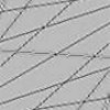
Higher-order statistics of natural images The implicit estimation of Wiener operators via polynomial kernels opens up new possibilities for the estimation of higher-order image statistics. Compared to the classical methods such as higher-order spectra, moments or cumulants, our approach avoids the combinatorial explosion caused by the exponential increase of the number of terms to be estimated and interpreted. When put into a predictive framework, multiplicative pixel interactions of different orders are easily visualized and conform to the intuitive notions about image structures such as edges, lines, crossings or corners. Arbitrarily oriented lines and edges, for instance, cannot be described by the usual pairwise statistics such as the power spectrum or the autocorrelation function: From knowing the intensity of one point on a line alone, we cannot predict its neighbouring intensities. This would require knowledge of a second point on the line, i.e., we have to consider some third-order statistics which describe the interactions between triplets of points. Analogously, the prediction of a corner neighbourhood needs at least fourth-order statistics, and so on.
This can be seen in the following experiment, where we decomposed various toy images into their components of different order.
The behaviour of the models conforms to our intuition: the linear model cannot capture the line structure of the image thus leading to a large reconstruction error which drops to nearly zero when a second-order model is used. Note that the third-order component is only
significant at crossings, corners and line endings.
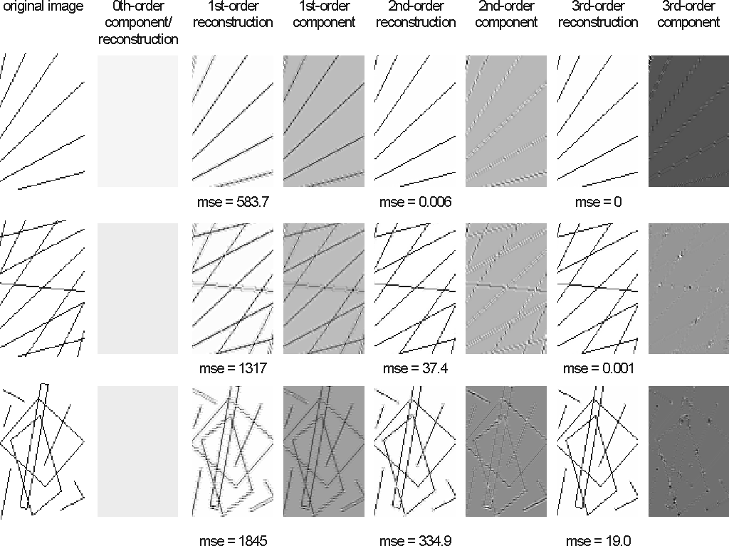
Pixel interactions up to the order of five play an important role in natural images. Here is an example decomposition:
Reference:
[4] Franz, M.O. and B. Schölkopf: Implicit Wiener series for higher-order image analysis. Advances in Neural Information Processing Systems 17, 465-472. (Eds.) Saul, L.K., Y. Weiss and L. Bottou, MIT Press, Cambridge, MA, USA (2005) [PDF].
Robust estimation with polynomial kernels
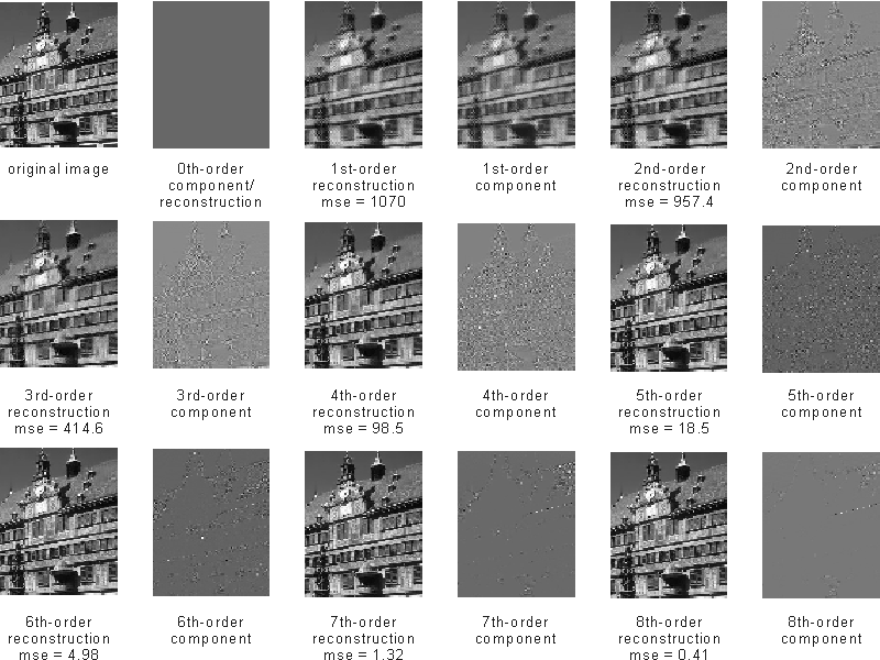
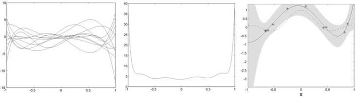
The use of a non-orthonormal function dictionary such as polynomials in ridge regression leads to a non-isotropic prior in function space. This can be seen in a simple toy example where the function to be regressed is a sinc function with uniformly distributed input and additive Gaussian noise. Our function dictionary consists of the first six canonical which are neither orthogonal nor normalized with respect to the uniform input. The effects on the type of functions that can be generated by this choice of dictionary can be seen in a simple experiment: we assume random weights distributed according to an isotropic Gaussian. In our first experiment, we draw samples from this distribution and compute the mean square of the for 1000 functions generated by the dictionary. It is immediately evident that, given a uniform input, our prior narrowly constrains the possible solutions around the origin while admitting a broad variety near the interval boundaries. If we do ridge regression with this dictionary (here we used a Gaussian Process regression scheme), the solutions tend to have a similar behaviour as long as they are not enough constrained by the data points (see the diverging solution at the left interval boundary). This can lead to bad predictions in sparsely populated areas.
We currently investigate alternative regularization techniques that result in an implicit whitening of the basis functions by penalizing directions in function space with a large prior variance. The regularization term can be computed from unlabelled input data that characterizes the input distribution. Here, we observe a different behaviour: the functions sampled from the prior show a richer structure with a relatively flat mean square value over the input interval. As a consequence, the ridge regression solution usually does not diverge as easily in sparsely populated regions near the interval boundaries.
Reference:
[5] Franz, M.O., Y. Kwon, C. E. Rasmussen and B. Schölkopf: Semi-supervised kernel regression using whitened function classes. Pattern Recognition, Proceedings of the 26th DAGM Symposium LNCS 3175, 18-26. (Eds.) Rasmussen, C. E., H. H. Bülthoff, M. A. Giese and B. Schölkopf, Springer, Berlin, Germany (2004) [PDF]